6-16-2025 The HVAC&R Weekly Edition: Issue #19

“TO AFFINITY AND BEYOND!” Exploring the nature of The Pump Affinity Laws.

As we move forward in our discussion regarding the addition of propylene glycol to a chilled water hydronic system, the natural progression of that dialogue leads to the obvious topic of Centrifugal Pump performance.

We’ve learned over the last couple of weeks, that adding glycol to a system can have a significant impact on a Chillers capacity by changing the solutions Specific Heat, Thermal Conductivity and Specific Gravity.

This week’s Session explores the changes to the solutions Specific Gravity and what impact that can have on a centrifugal pump. First we need to develop a foundation to base our conclusions on by using a defined set of rules or laws for predicting pump performance.

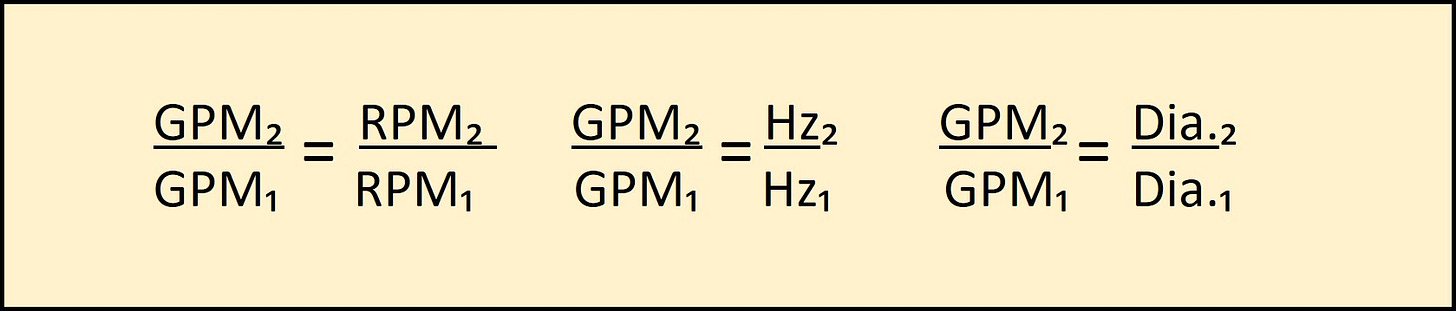
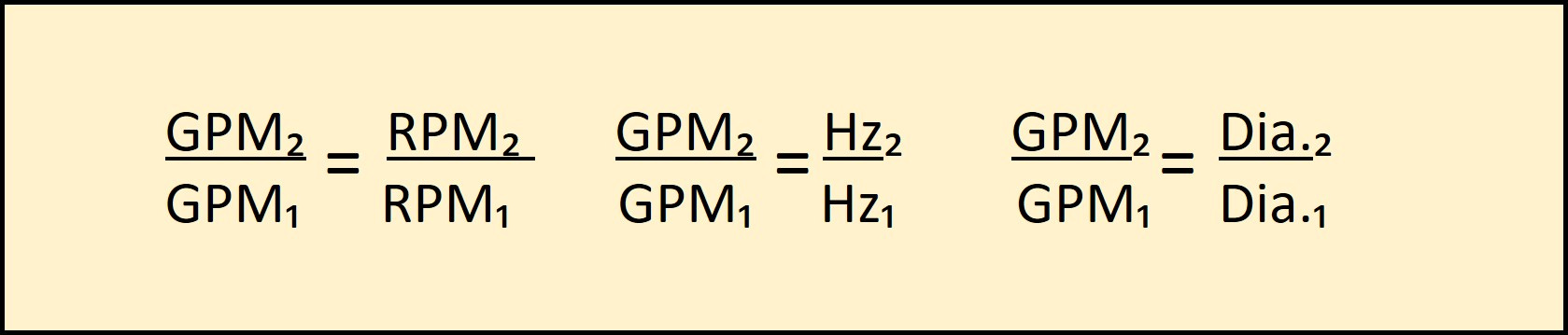
THE PUMP AFFINITY LAWS

1. The G.P.M. (Q) is directly proportional to speed (N) or impeller Diameter (D).

   

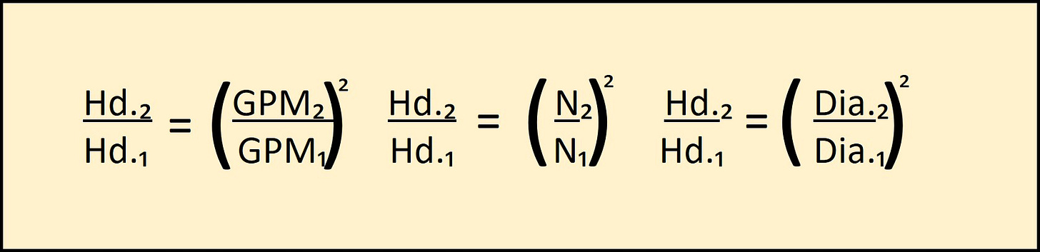
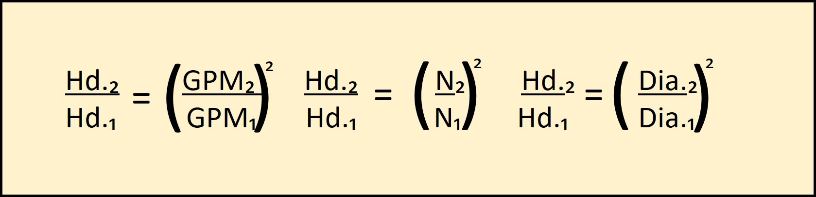
2. The Ft.-Hd. (Hd.) varies to the square of the G.P.M. (Q), speed (N), or Diameter (D)

   

3. Brake Horsepower (P) varies to the cube of the G.P.M. (Q), Speed (N),

   Diameter (D).

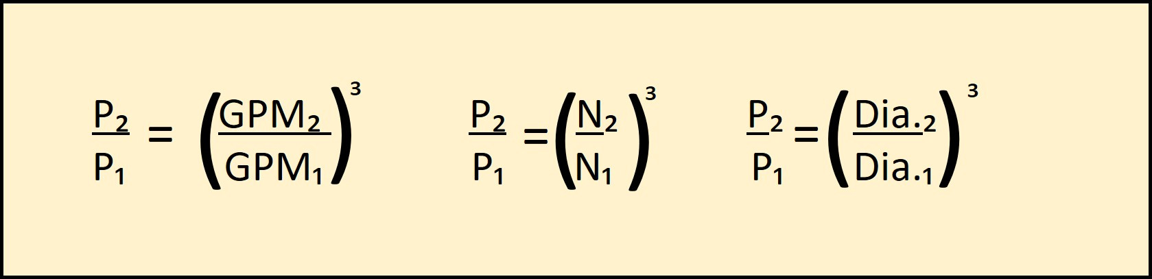
If the density of a fluid is changed it changes The Affinity Law for that application.

Maybe a brief clarification on what Water Horsepower and Brake Horsepower describes would be helpful.

Water Horsepower (W.H.P.) is just what it suggests. It’s the theoretical energy required to move, lift, or circulate water through a circuit based on its Specific Gravity and flow rate, while circulating against the Ft.-Hd. pressure drop of the system. It does not take into account for pump and motor efficiency losses. The circuit maybe a closed loop system like a chilled water circuit, or an open loop system like a condenser water circuit going to a cooling tower.

Brake Horsepower is the energy required to move a water solution through a circuit after taking pump and motor efficiency losses into account. Brake Horsepower (B.H.P.) is always going to be greater than Water Horsepower (W.H.P.) because of those losses. Think of B.H.P. as the power required of the motor to turn the shaft of the pump to drive a liquid through a piping system. To figure the W.H.P. and B.H.P. several fundamental data points should be reviewed first.

DATA POINTS RELATED TO PURE WATER AND WORK:

1. Density of Water: 62.4 Lbs./cu.ft. (for this discussion)

2. Density of Water: .0361 lbs./cu.in. (62.4 Lbs./cu.ft. ÷ 1,728 cu.in./cu.ft. = 0.0361)

3. One Gallon of Water: 231 Cu.in.

4. Gallons in 1 cubic ft. of water: 7.48 Gals. (1728 Cu.in./cu.ft. ÷ 231 cu.in./gals. = 7.48 gals.)

5. Weight of 1 gallon of water : 8.33 lbs. (62.4 lbs. ÷ 7.48 gals. ≈ 8.33 Lbs./gals.) or (231 cu.in./gal. x .0361 lbs./cu.in. = 8.33 lbs./gal.)

6. Specific Gravity of Water: 1.0 (Sp. Gr.)

7. PSI per Ft.-Head of Water: .433 psi/ft. (62.4 lbs./cu.ft. ÷ 144 sq.in/sq.ft. = .433 psi) or (12” x .0361 lbs./cu.in. = .433 psi/ft.)

8. Ft.-Hd. of water per 1 PSI: 2.31 Ft.-Hd. (1 PSI ÷ .433 PSI/Ft. = 2.31 ft.)

9. 1 Horsepower: 550 Ft.-lbs./sec. (Something about an English Dray Horse)

10. 1 Horsepower: 33,000 Ft.-lbs./min. (550 Ft.-Lbs. x 60sec./minute)

11. 3960: A constant for finding W.H.P. using G.P.M. and ∆Ft.-Hd. (33,000 ÷ 8.33 ≈ 3960) by factoring in pump and motor efficiencies we can determine B.H.P.

12. 1714: A constant for finding W.H.P. using G.P.M. and ∆P.S.I.D. 33,000 ÷ (8.33 x 2.31) ≈ 1714] by factoring in pump and motor efficiencies we can determine B.H.P.

There are two formulas that we should look at to find the required W.H.P. and B.H.P.

WATER HORSEPOWER FORMULA

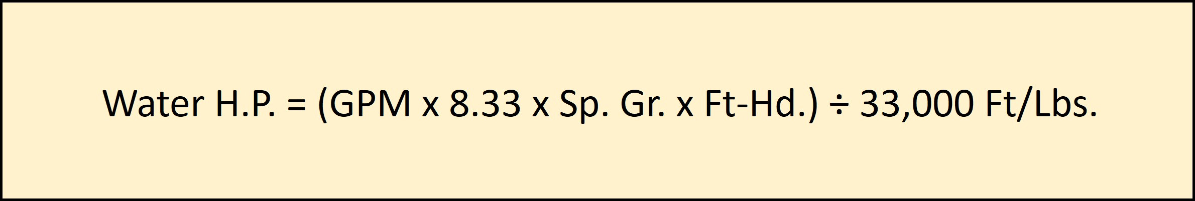
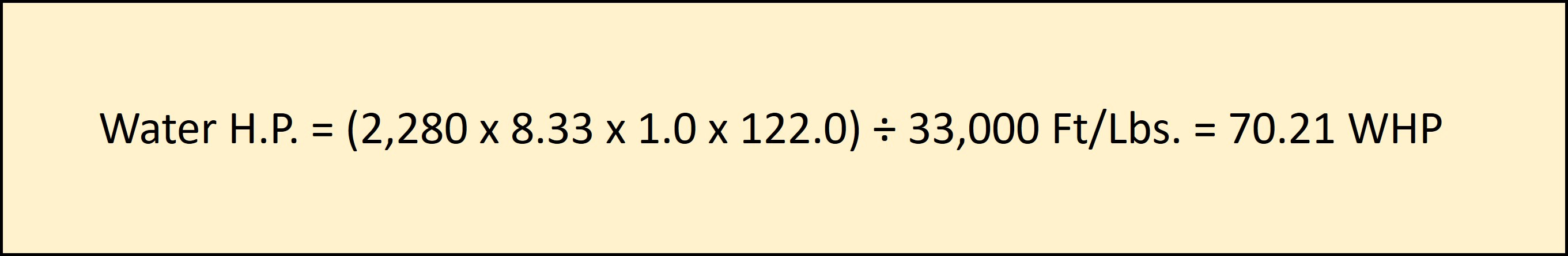
If we take the original design G.P.M. of 2,280, and the 22 ∆Ft.-Hd. for the chiller + 100 Ft.-Hd. for the system loop (122 ∆Ft.-Hd. Total) we find the W.H.P. for pure water is:

BRAKE HORSEPOWER FORMULA

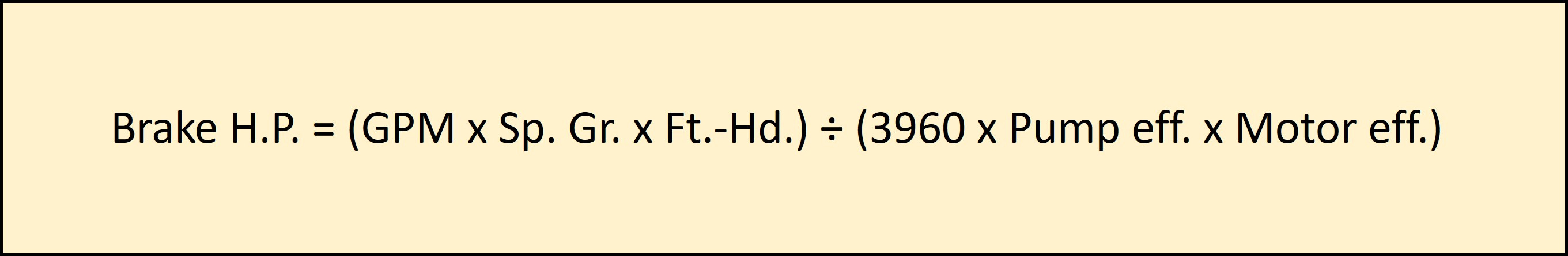
This formula takes the pump and motor efficiencies into account. We can use the Constant 3960 in the calculation for ∆Ft.-Hd. (Note they remove the 8.33 from the formula when using 3960).

Here is the Brake H.P. when we include the Pump Eff. of .80 and Motor Eff. of .95

We can see the pump motor requires a selection for a 100 M.H.P. (Motor Horse Power) rating to meet the Design G.P.M. and ∆Ft.-Hd. for pure water.

SO, THE RUMORS ARE TRUE!

Lets see what happens with that selection when we add the glycol and increase the flow to 2,462 G.P.M. using 26.7 ∆Ft.-Hd. for the chiller + 104 ∆Ft.-Hd. for the system loop (130.7 ∆Ft.-Hd. Total) and a Specific Gravity of 1.035. This is based on our analysis from last week

With The 110.6 B.H.P. requirements, the full impact comes into view. The increases in G.P.M., ∆Ft.-Hd. pressure drop, and Specific Gravity, required to meet system capacity, can have significant consequences on the power requirements for the pump motor.

To meet this new horsepower requirement would mean selecting a larger motor capacity (125 M.H.P.), assuming that configuration for that pump is available. An assessment of the M.C.C. Panel, wire size, as well as V.F.D. sizing (if applicable), and any deratings for elevation that might be required.

If the flow was kept at the original 2,280 G.P.M. and 126.7 ∆Ft.-Hd. (Total) for glycol, the B.H.P. would increase to 106.6 B.H.P.

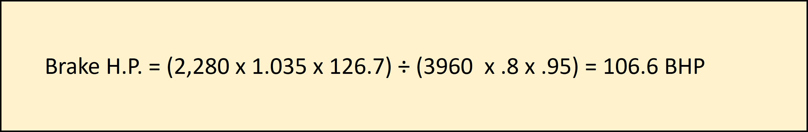
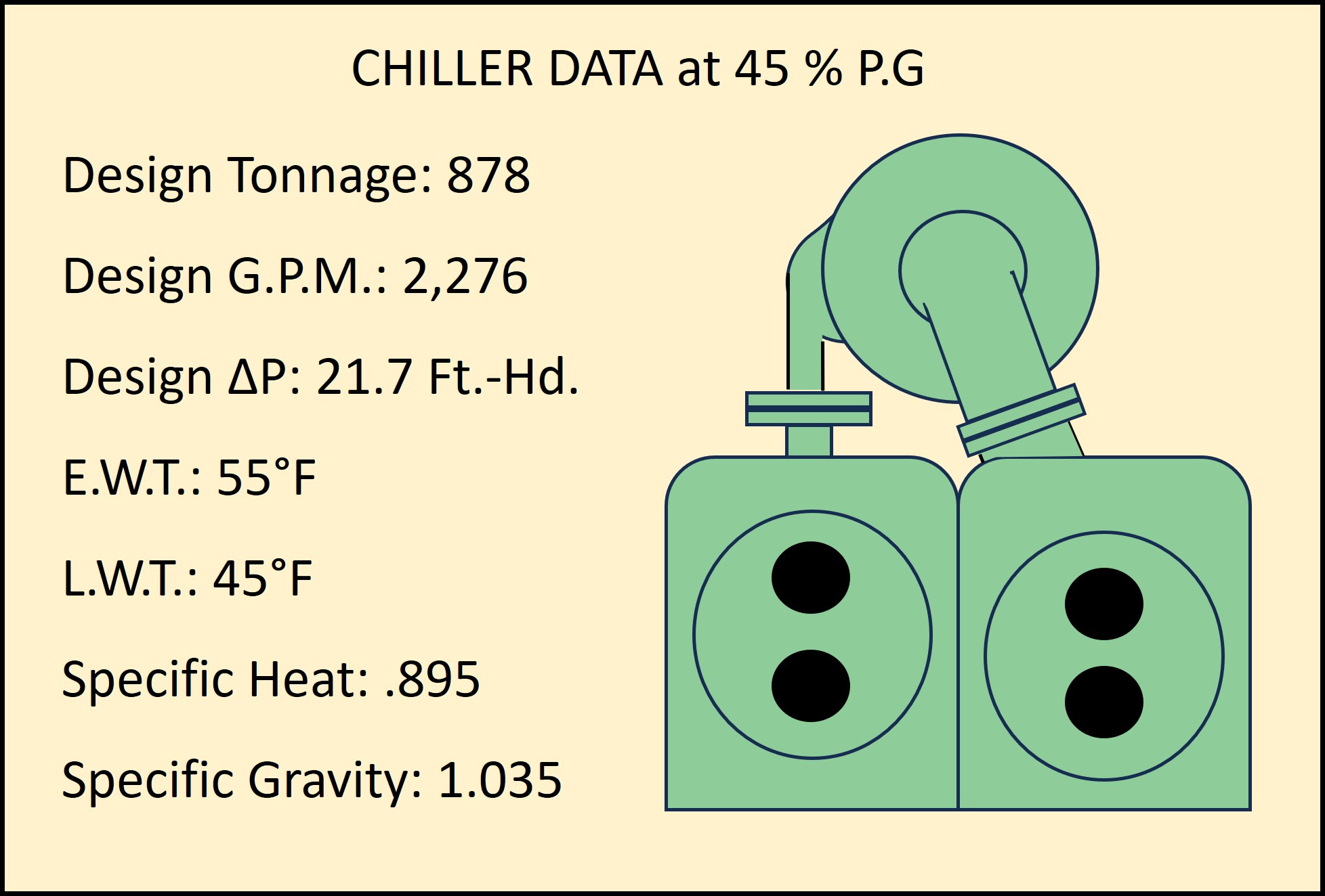
This is still over the original 100 M.H.P. requirement so a new motor would still be in order, and we are still left facing the 7.6% loss in Chiller capacity. In order to keep the pump M.H.P. below 100 H.P. we would need to reduce the GPM slightly to 2,276 and pressure drop using 21.7 Ft.-Hd. for the chiller + and 100.3 Ft.-Hd. for the system loop (122. Ft.-Hd. Total)

This lower G.P.M. and pressure drop results in a capacity reduction of the chiller to 878 Tons roughly a loss of 72 Tons+/- or 7.6 %. Is that acceptable? I don’t know.

The point of this study was to bring light to the importance of analyzing and understanding the ramifications of adding glycol to a system after the equipment selection process was completed, approved, purchased, and installed, especially without “running” the numbers first.

By analyzing the data we can see the impact on the Chiller’s performance but, also on the associated electrical service, pump(s,) and Heat Transfer Devices in the loop.

Next week let’s look at some pump curves, and study how Series and Parallel pumping play out. We can discover how we can develop at System Pump Curve, and explore what primary-secondary pumping looks like.

Until next week be happy and be safe!

See Previous Issue